Tutorial

This is a tutorial to get you started using PyOpenCAP. Here, we walk through the steps to generate the zeroth order Hamiltonian and the CAP matrix required to perform a perturbative CAP/XMS-CASPT2 calculation on the \({}^2\Pi_g\) shape resonance of \(N_2^-\).

To follow along with the tutorial, install PyOpenCAP, clone the repository, and open a Python interpreter in the examples/pyopencap/openmolcas directory. Alternatively, copy the files “nosymm.rassi.h5” and “nosymm.out” located in the examples/opencap directory to your working directory, and set the “RASSI_FILE” and “OUTPUT_FILE” variables to the appropriate paths.

A notebook version of this tutorial can be found here.

Preliminary: Importing the module

In addition to PyOpenCAP, we’ll import numpy to help us process the data. We’ll also set the paths to the RASSI_FILE and OUTPUT_FILE generated by OpenMolcas, which we’ll be processing to run our perturbative CAP calculation.

>>> import pyopencap
>>> import numpy as np
>>> RASSI_FILE = "../../opencap/nosymm.rassi.h5"
>>> OUTPUT_FILE = "../../opencap/nosymm.out"

Constructing the System object

The System object of PyOpenCAP contains the geometry and basis set information, as well as the overlap matrix. The constructor takes in a Python dictionary as an argument, and understands a specific set of keywords . There are three equivalent ways of specifying the geometry and basis set: rassi_h5, molden, and inline. Here, we’ll use the rassi_h5 file.

>>> sys_dict = {"molecule": "molcas_rassi","basis_file": RASSI_FILE}
>>> s = pyopencap.System(sys_dict)
>>> smat = s.get_overlap_mat()
>>> np.shape(smat)
Number of basis functions:119
(119, 119)

Constructing the CAP object

The CAP matrix is computed by the CAP object. The constructor requires a System object, a dictionary containing the CAP parameters, the number of states (10 in this case), and finally the string “openmolcas”, which denotes the ordering of the atomic orbital basis set.

>>> cap_dict = {"cap_type": "box",
        "cap_x":"2.76",
        "cap_y":"2.76",
        "cap_z":"4.88",
        "Radial_precision": "14",
        "angular_points": "110"}
>>> pc = pyopencap.CAP(s,cap_dict,10,"openmolcas")

Parsing electronic structure data from file

The read_data() function can read in the effective Hamiltonian and densities in one-shot when passed a Python dictionary with the right keywords. For now, we’ll retrieve the effective Hamiltonian and store it as h0 for later use.

>>> es_dict = {"method" : "ms-caspt2",
       "molcas_output":OUTPUT_FILE,
       "rassi_h5":     RASSI_FILE}
>>> pc.read_data(es_dict)
>>> h0 = pc.get_H()

Passing densities in RAM

Alternatively, one can load in the densities one at a time using the add_tdms() or add_tdm() functions. We load in the matrices from rassi.h5 using the h5py package, and then pass them as numpy arrays to the CAP object. In this example, the CAP matrix is made to be symmetric.

>>> import h5py
>>> f = h5py.File(RASSI_FILE, 'r')
>>> dms = f["SFS_TRANSITION_DENSITIES"]
>>> pc = pyopencap.CAP(s,cap_dict,10,"openmolcas")
>>> for i in range(0,10):
>>>     for j in range(i,10):
>>>         dm1 = np.reshape(dms[i][j],(119,119))
>>>         pc.add_tdm(dm1,i,j,"openmolcas",RASSI_FILE)
>>>         if i!=j:
>>>             pc.add_tdm(dm1,j,i,"openmolcas",RASSI_FILE)

Once all of the densities are loaded, the CAP matrix is computed using the compute_perturb_cap() function. The matrix can be retrieved using the get_perturb_cap() function.

>>> pc.compute_perturb_cap()
>>> W_mat=pc.get_perturb_cap()

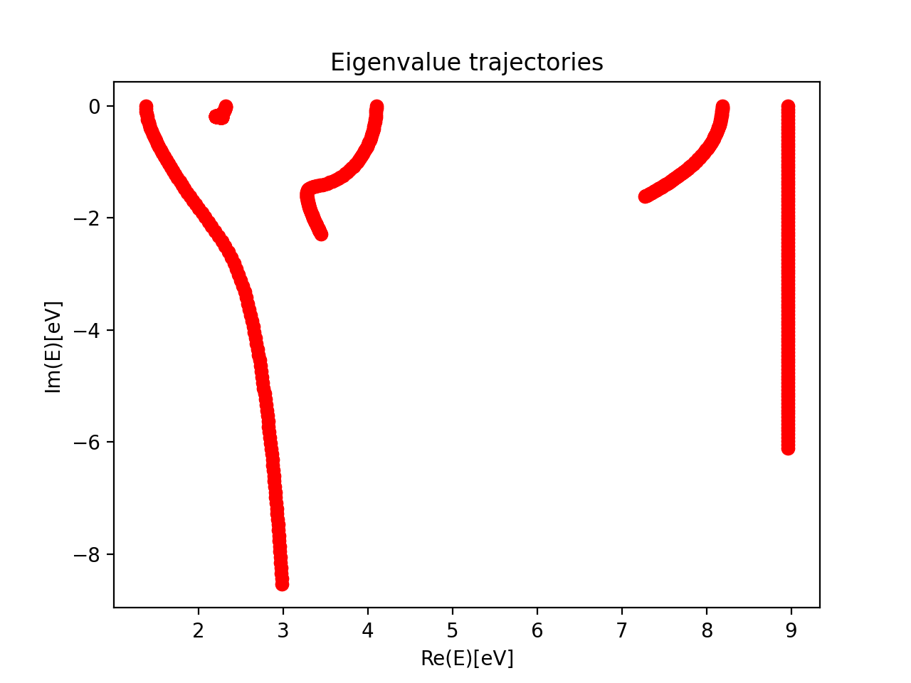
We now have our zeroth order Hamiltonian (stored in h0) and our CAP matrix(W_mat) in the state basis. Extracting resonance position and width requires analysis of the eigenvalue trajectories.

The script example.py runs this example and diagonalizes the CAP-augmented Hamiltonian \(H^{CAP}=H_0-i\eta W\) over a range of \(\eta\)-values. The reference energy was obtained in a separate calculation which computed the ground state of the neutral molecule with CASCI/CASPT2 using the optimized orbitals of the anionic state. The results are plotted below:

The resonance trajectory will vary slowest with the changing CAP strength. Zooming in on the trajectory near 2.2eV, we also plot the “corrected” trajectory, which is obtained by applying the first-order correction:

\(U(\eta)=E(\eta)-\eta\frac{\partial E(\eta) }{\partial \eta}\).

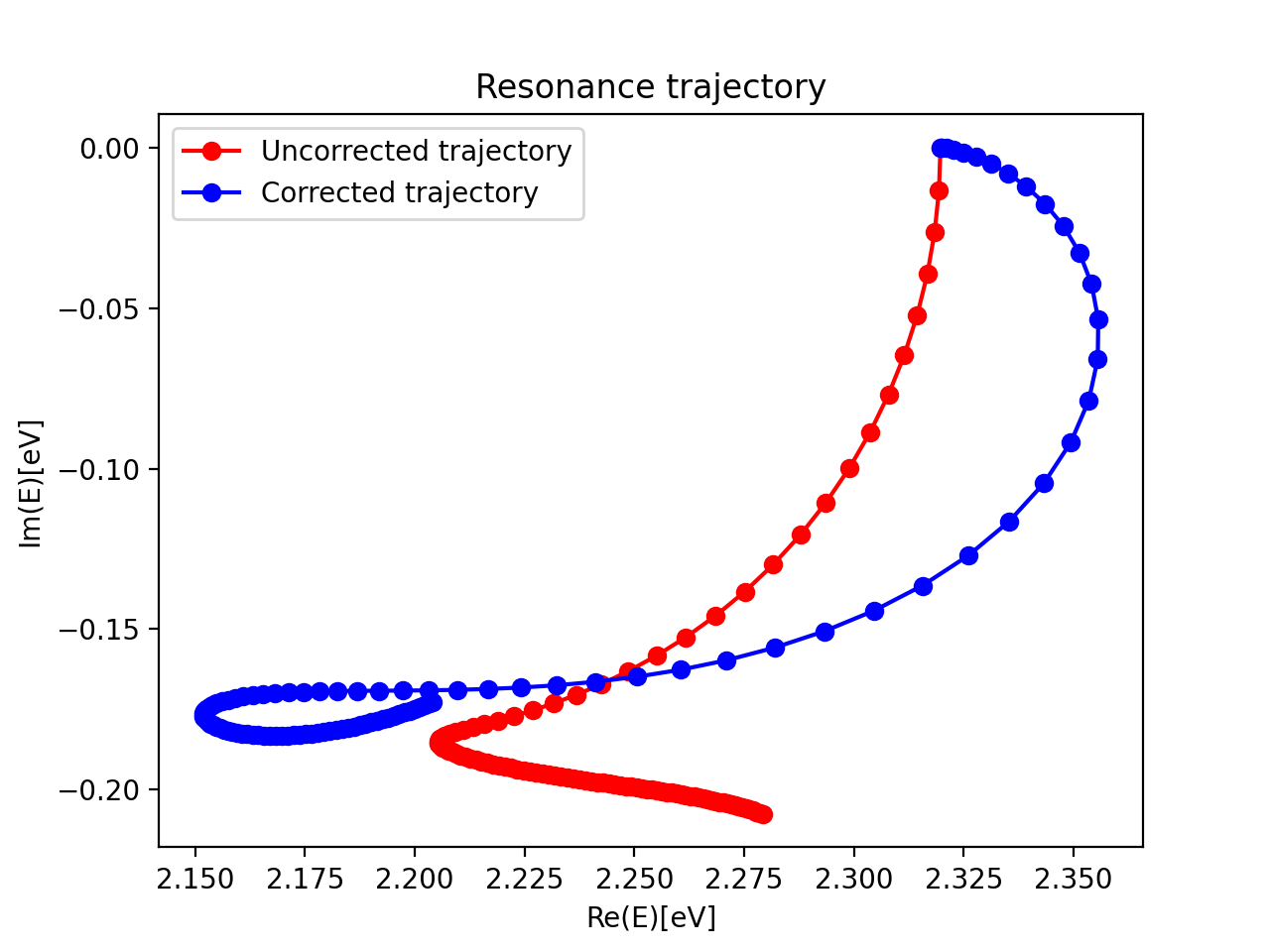
Finally, the best estimate of resonance position and width are obtained at the stationary point

\(\eta_{opt} = min \left | \eta^2 \frac{\partial^2 E }{\partial \eta^2} \right |\).

For this example, this yields a resonance energy of 2.15eV, and a width of 0.35eV.